I've recently been experimenting with Data Visualisation in R. As part of that I've put together a little bit of (probably error ridden and redundant) code to help mapping of Australia.
First, my code is built on a foundation from [Luke's guide to building maps of Australia in R](http://lukesingham.com/map-of-australia-using-osm-psma-and-shiny/), and [this guide to making pretty maps in R](https://timogrossenbacher.ch/2016/12/beautiful-thematic-maps-with-ggplot2-only/).
The problem is that a lot of datasets, particularly administrative ones, come with postcode as the only geographic information. And postcodes aren't a very useful geographic structure - there's no defined aggregation structure, they're inconsistent in size, and heavily dependent on history.
For instance, a postcode level map of Australia looks like this:
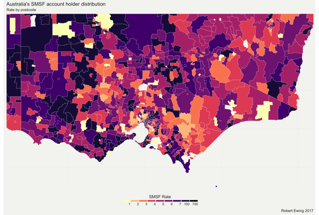
Way too messy to be useful.
The ABS has a [nice set of statistical geography](http://www.abs.gov.au/AUSSTATS/abs@.nsf/Lookup/1270.0.55.001Main+Features1July%202016?OpenDocument) that will let me fix this problem by changing the aggregation level, but first I need to convert the data into another file.
Again, fortunately the ABS publishes concordances between postcodes and the Statistical Geography, so all I need to do is take those concordances and use them to mangle my data lightly. First, I used those concordances to make some CSV input files:
Postcode to Statistical Area 2 level (2011)
Concordance from SA2 (2011) to SA2(2016)
Statistical Geography hierarchy to convert to SA3 and SA4
Then a little R coding. First convert from Postcode to SA2 (2011). SA level 2 is around the same level of detail of postcodes, and so the conversions won't lose a lot of accuracy.And then convert to 2016 and add the rest of the geography:
## Convert Postcode level data to ABS Statistical Geography heirarchy
## Quick hack job, January 2017
## Robert Ewing
require(dplyr)
## Read in original data file, clean as needed.
## This data file is expected to have a variable 'post' for the postcode,
## and a data series called 'smsf' for the numbers.
data_PCODE <- read.csv("SMSF2.csv", stringsAsFactors = FALSE)
## Change this line depending on your data series.
## This code is designed to read in only one series. If you need more than one,
## you'll need to change the Aggregate functions.
## Change this line to reflect the name of the data series in your file
data_PCODE$x <- as.numeric(data_PCODE$smsf)
data_PCODE$smsf[is.na(data_PCODE$x)] <- 0
data_PCODE$POA_CODE16 <- sprintf("%04d", data_PCODE$post)
## Read in concordance from Postcode to SA2 (2011)
concordance <- read.csv("PCODE_SA2.csv", stringsAsFactors = FALSE)
concordance$POA_CODE16 <- sprintf("%04d", concordance$POSTCODE)
## Join the files
working_data <- concordance %>% left_join(data_PCODE)
working_data$x[is.na(working_data$x)] <- 0
## Adjust for partial coverage ratios
working_data$x_adj = working_data$x * working_data$Ratio
## And produce the SA2_2011 version of the dataset. Data is in x.
data_SA2_2011 <- aggregate(working_data$x_adj,list(SA2_MAINCODE_2011 = working_data$SA2_MAINCODE_2011),sum)
## Now read in the concordance from SA2_2011 to SA2_2016
concordance <- read.csv("SA2_2011_2016.csv", stringsAsFactors = FALSE)
## Join it.
working_data <- concordance %>% left_join(data_SA2_2011)
working_data$x[is.na(working_data$x)] <- 0
## Adjust for partial coverage ratios
working_data$x_adj = working_data$x * working_data$Ratio
## And produce aggregate in SA2_2016
data_SA2_2016 <- aggregate(working_data$x_adj,list(SA2_MAINCODE_2016 = working_data$SA2_MAINCODE_2016),sum)
## and finally join the SA2 with the rest of the hierarchy to allow on the fly adjustment.
statgeo <- read.csv("SA2_3_4.csv", stringsAsFactors = FALSE)
data_SA2_2016 <- data_SA2_2016 %>% left_join(statgeo)
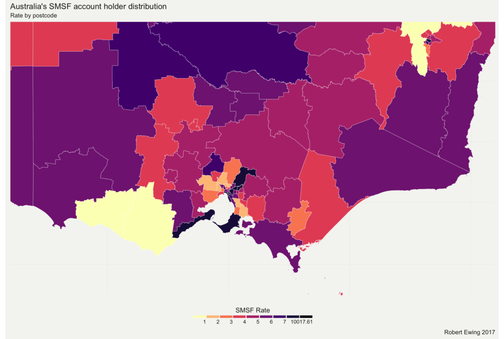
The end result gives you a data set that can be converted to a higher level. Here's the chart above, but this time using SA3 rather than postcodes: